Discreet Deconvolution using Linear Algebra

Deconvolution is the action of recovering a signal before it has been convoluted. In the context of images, this would be taking a blurred image and recovering a sharper one (and not just artificially but actually recovering the spread out information).

A common simple example to demonstrate deconvolution is by using some tricks of Fourier transforms. However, I will take a mathematically even simpler concept and just use linear algebra. The discreet convolution operation can be constructed as a matrix multiplication:

Ax=b

Where A is a Toeplitz matrix (all diagonal elements are the same) representing the convolution operation, x is the signal I want to recover, and b is the convoluted data I have. If A is invertable (it might not be), I can multiply both sides by its inverse to get the solution for x:

A^-1Ax=A^-1b
x=A^-1b

What does A look like? Each row of the matrix A have the same set of values but are shifted one index to the right for each subsequent row. For example, to represent the convolution by a boxcar function I would have A matrix like this:

def boxcar(ir,L):
    y = numpy.zeros(L)
    y[:ir]=1
    y[-ir+1:]= 0 if ir==1 else 1
    return y

A = [numpy.roll(boxcar(2,7),i) for i in range (7)]

The diagonals are all 1, meaning that after a multiplying it with the x, it returns the original value, and the element on either side of the diagonal is also 1, meaning that now the new value is a sum of the original value plus the two adjacent to it. Note that in this example I formulate it as a circulant matrix. Now if we are lucky this matrix is invertable – and indeed it is!

A-1=[[ 1 1 -2 1 1 -2 1]
[ 1 1 1 -2 1 1 -2]
[-2 1 1 1 -2 1 1]
[ 1 -2 1 1 1 -2 1]
[ 1 1 -2 1 1 1 -2]
[-2 1 1 -2 1 1 1]
[ 1 -2 1 1 -2 1 1]]/3

Here the number 3 is just the determinant of A. Note that the presence of negative numbers alludes to differentiation operations. Interesting thing to note in the inverted matrix is that 3A^-1 contains the exact same value of A plus a pattern of -2, 1, 1, -2 in reach row. Demonstrating deconvolution – if I have

b=[0 0 1 1 1 0 0]
then
x=A^-1b=[0 0 0 1 0 0 0]

This example is special since the matrix b is also the same as the convolution kernel (the one that is shifted around to make the matrix A). The following graphic shows a more complex example where there is more structure to the restored signal:

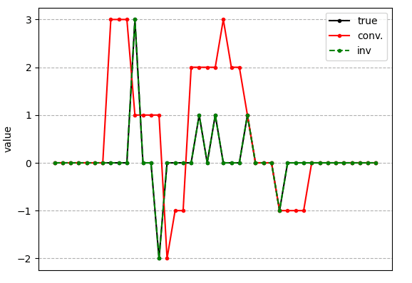
It can solve easily! Now lets introduce noise into the system (which is a more realistic scenario when dealing with real data):

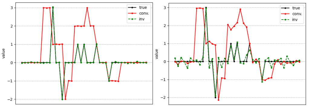
Clearly the deconvolution does not restore perfectly due to the addition of Gaussian noise on top of the convoluted signal (i.e. not before convolution on the true signal). This makes sense because if we introduce noise into our matrix equation x’=A^-1(b+noise) we get x’=A^-1b+A^-1noise=x+A^-1noise. So the deconvoluted signal has an additional A^-1noise distribution on top of the true signal x.

To do this yourself you can get my Python code here.

Technical details

As it turns out, there are a number of methods that can be used to solve Ax=b and surprisingly the inverted matrix example is not the most accurate (unless it is solved algebraically). In the following graphic it can be seen, if we consider the difference between the deconvoluted signal and the true signal, that the numpy routine solve actually gives the most accurate result. Additionally, I included the fast Fourier transform method, which works quite well in this example too.

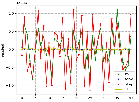
However! If I introduce noise into the system…

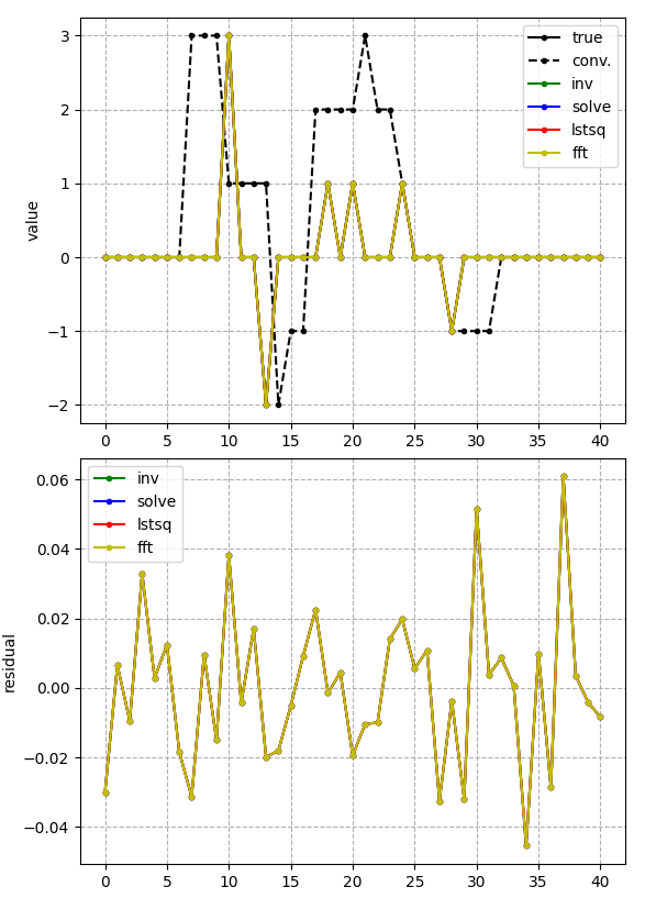
Now the residual error for all method is effectively the same! I don’t know why this is so, presumably it is because all methods solve the same problem and the only difference between them is at the machine precision level so including noise in the system creates a residual at a level much greater obscuring the difference in the methods.

• WordPress
• YouTube
• GitHub