Simple model of real-world data in Python

The purpose of computation is insight, not numbers.
Richard Hamming

In this post I will show you how to make a simple (yet potentially insightful) model of a complex phenomenon observed in the real-world. To such end, I will use the recent COVID-19 Coronavirus Outbreak for our modelling exercise. But first, a short background…

Short background

One rabbit, 3 rabbits, 9 rabbits, 27 rabbits, …. this sequence represents exponential growth of a population (given that each rabbit creates 2 more rabbits per iteration). The way infectious diseases spread also exhibits exponential growth. Mathematically this can be represented as the differential equation $\frac{dP(t)}{dt} = rP(t)$ , where $P(t)$ is the population at time $t$ and $r$ is the rate constant. When the rate constant is positive the population will exponentially grow; if its negative then it exponentially decays. A simple exponential function satisfies the above differential equation: $P(t) = P(0)e^{rt}$ where $P(0)$ is the population at the beginning of time, $t=0$ . Evidently, this model is too ambitious as the population will tend to infinity over time.

In reality, the population will saturate due to the natural limits of the environment. To reflect this, the differential equation above is modified by the term $1- P(t)/K$ and we get: $\frac{dP(t)}{dt} = rP(t)(1-P(t)/K)$ where $K$ is the maximum possible population (also known as the carrying capacity). This differential equation also has a solution: $P(t) = \frac{KP(0)}{P(0)-(K-P(0))e^{-rt}}$ . This form is known as the logistic function. Compare the two models below:

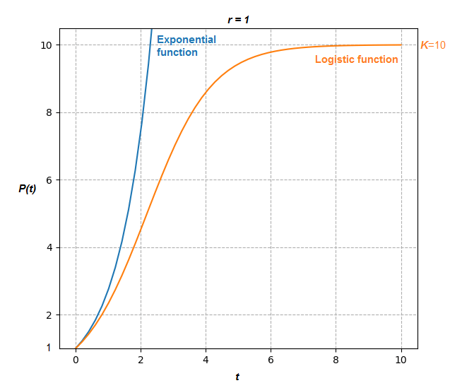
Clearly the population stabilizes at the value $P=10$ in this example for the Logistic function with $K=10$ , whereas the exponential function tends to infinity.

Infection model

For modelling the case of the COVID-19 Coronavirus Outbreak we want to fit the available data and determine when the infection started, when it will end, and how many people will be infected.

Disclaimer: this is merely an exercise and should not be considered as any meaningful predictions

So lets start by defining the following relevant variables:

$P(t)$ is the number of active infected cases (can still infect others) at a given time,
$P_{new}(t)$ is the number of new infected cases at a given time,
$P_{closed}(t)$ is the number of closed cases at a given time, i.e. they can no longer spread the infection (either healed or dead), and
$P_{total}(t)$ is the sum total of infected cases over time.

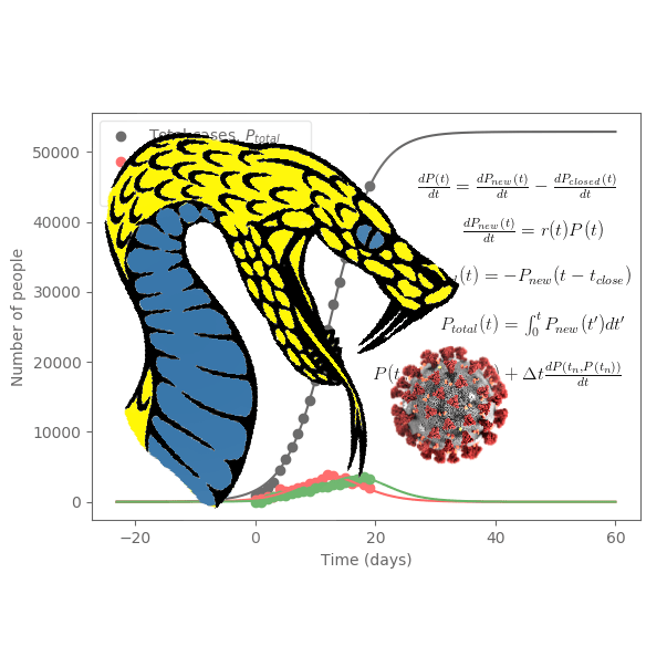
Using the above variables we construct four equations:

$\frac{dP(t)}{dt} = \frac{dP_{new}(t)}{dt} - \frac{dP_{closed}(t)}{dt}$

the change in the active infected cases is equal to the change of new infected cases minus the change of closed cases.

$\frac{dP_{new}(t)}{dt} = r(t)P(t)$

this is the exponential growth part; new infected cases grow with increasing active infected cases.

$P_{closed}(t) = -P_{new}(t-t_{close})$

closed cases are just equal the the new cases at a later time $t_{close}$ . In other words, once infected it takes time $t_{close}$ until they recover (or die).

$P_{total}(t) = \int_{0}^{t} P_{new}(t') dt'$

by integrating the new cases we can get the total number of infected cases.

Note that in the second equation we have $r(t)$ which is the rate constant as a function of time. In reality, the more people have been infected the less people there are to infect, therefore the rate constant would start high and end low, much like the logistic function in a population growth model. Therefore, we use the following equation for the rate constant: $r(t) = r_0(1-P_{total}(t)/P_{total,max})$ where $r_0$ is the rate constant at $t=0$ and $P_{total,max}$ is the maximum possible total number of cases. So when the total number of cases is equal to the maximum possible cases the rate constant is zero so new infections stop.

Solving the differential equation

We want to calculate $P_{total}(t)$ , $P_{new}(t)$ , and $P_{closed}(t)$ for fitting the available data. To do so we need to calculate $P(t)$ first, which is a differential equation. As compared to simple exponential growth or the logistic function the differential equation can not be easily solved analytically so we will use numerical integration. In this case we will use a simple Euler method:

$P(t_{n+1}) = P(t_n) + \Delta t\frac{dP(t_n,P(t_n))}{dt}$ ,

where $n$ is the index of the time step and $\Delta t$ is the size of the time step (the smaller the more accurate but takes longer to compute over a given time interval). In Python it will look as follows: P_curr = P[-1] + dt*dPdt[-1]. Here I decided to append the lists P and dPdt each iteration, so the most recent time is at the last index, which is accessed by [-1].

The model and its solution can then be defined in Python as follows:

import numpy as np
def Infection_model(t_in,t0,t_close,r0,K):
    """
    t_in     : time at which to calculate [day]
    t0       : time at which infections started [day]
    t_close  : time until no longer infectious (closed case) [day]
    r0       : initial infection rate constant [/day]
    K        : maximum possible total number of cases (or carrying capacity)
    """
    # Model Parameters
    dt = 1/400 #Time step (Smaller is more accurate) [days]
    P0 = 1 #Initial infected population (always starts at 1)
    t_a = np.arange(0,t_in.max()+t0,dt) #Time range to calculate [days]

    # Define initial conditions and lists
    P, dPdt = ([P0],[0])
    P_new_list, P_closed_list = ([0],[0])
    P_total_cases_list = [P0]
    
    # Calculate
    for ind,t in enumerate(t_a): #For each time
        r = r0*(1-P_total_cases_list[-1]/K) #Infection rate constant (q used as "carrying capacity") [/day]
        dP_new = r*P[-1] #rate of new infected cases [/day]
        dP_closed = np.interp(t-t_close,t_a[:ind+1],P_new_list) if t >= t_close else 0 #rate of closed cases [/day]
        P_total_cases = P_total_cases_list[-1]+dt*dP_new #Current number of total cases
        
        #Numerical difference time stepping
        dPdt_curr = dP_new - dP_closed  #Change in population for current step [/days]
        P_curr = P[-1] + dt*dPdt[-1] #Population for current step (forward Euler method)
            
        #Append arrays
        P.append(P_curr)
        P_total_cases_list.append(P_total_cases)
        dPdt.append(dPdt_curr)
        P_new_list.append(dP_new)
        P_closed_list.append(dP_closed)
        
    t_a = np.append(t_a,t_a[-1]+dt) #Include the time for the last calculated point as well
    return P_new_list, P_closed_list, P_total_cases_list, t_a

A lot of it is self-explanatory with the comments. One noteworthy thing is that for calculating closed cases I use a linear interpolation routine. This is necessary for the curve fitting algorithm because there needs to be a finite change in the objective function with a change in the parameter t_close (this is evidenced by the result that the estimated value is the same as the guessed value). Otherwise, for plotting simply using P_new_list[-int(t_close // dt + 1)] instead of np.interp(...) is much faster.

Data fitting

Lets have a look at the available data that we want to fit:

We want to fit not only the total cases but the new cases and closed cases as well because those parameters will provide more information about the rate constant $r_0$ and $t_{closed}$ , respectively. Note in the above graph that at Time = 0 it’s on January 22, 2020. Also, I truncated the data after the classification method changed that caused a large spike in total cases. Furthermore, the closed cases is an estimate given by the deaths divided by the fatality rate (used 0.03).

To fit the data we will use the scipy routine curve_fit. This routine minimizes the sum of squared residuals for non-linear functions with respect to the fitting parameters (also called non-linear least squares). The first three arguments are the model function (Infection_model(t_in,t0,t_close,r0,K)), the independent variable (time), and the dependent variable. The dependent variable here is $P_{total}(t)$ , $P_{new}(t)$ , and $P_{closed}(t)$ . The trick to fit all of them simultaneously is to combine the three lists (or numpy arrays) into a single list before feeding it into the curve fitting routine. Therefore, we define another function that is used specifically for the fitting routine:

def Infection_model_fit(t_in,t0,t_close,r0,K):
    P_new_list, P_closed_list, P_total_cases_list, t_a = Infection_model(t_in,t0,t_close,r0,K)
    #Interpolate to get points exactly at time t_in
    P_total_cases_list = np.interp(t_in+t0,t_a,P_total_cases_list)
    P_new_list = np.interp(t_in+t0,t_a,P_new_list)
    P_closed_list = np.interp(t_in+t0,t_a,P_closed_list)
    return np.append(P_total_cases_list,np.append(P_new_list,P_closed_list)) #Three arrays appended into one for fitting

Note how I append the three arrays together into one. Now we can call the curve fitting routine as follows:

day = np.arange(0,len(tot_cases)) #Time [day]
pguess = [20,7,0.4,8e4] #Guess parameters for the fitting routine [t0,t_close,r0,K]
popt, pcov = curve_fit(Infection_model_fit, day, np.append(np.append(total_cases,daily_cases),closed_cases), pguess)

popt is the optimally determined parameters for minimizing the least-squares and pcov is the covariance matrix of those parameters, which we will use to estimate the error in the parameters later. Again, note how the input data is appended into a single array. The result of the fitting is as follows:

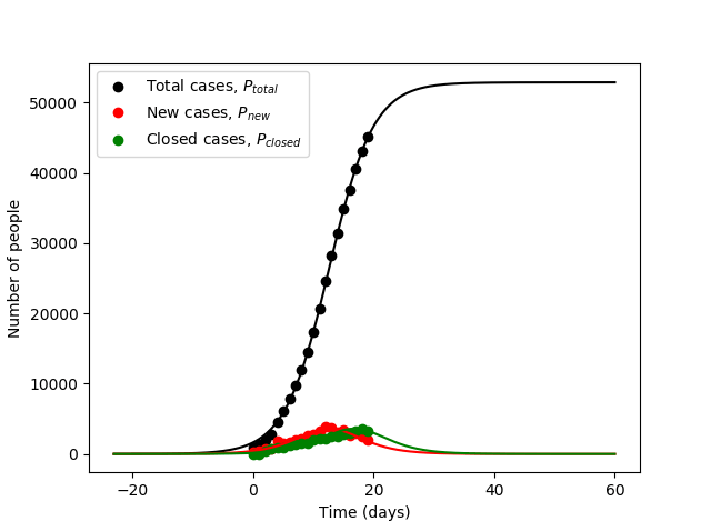
Looks good! The optimal parameters are determined as follows:

Time when the infection started, $t_0 = 23.1 \pm 0.6$ days (before 1st measured data)
Time until closed case, $t_{close} = 4.2 \pm 0.4$ days
Initial infection rate constant, $r_0 = 0.402 \pm 0.019$ /day
Maximum possible total number of cases (or the carrying capacity), $P_{total,max} = 77893 \pm 4282$

What can we get from this?

First of all, the 1st measured data was on January 22, 2020, and given the estimate of $t_0$ we can guess that the first infection was 23.1 days before then, which would make it on December 30, 2019. Internet sources say the first cases were known in December but the very first could have been in November or earlier.

The estimate of the transmission rate $R_0$ (number of people an infected person will infect by the time they are no longer infectious) is given by $t_{close} \times r_0$ , which gives 1.68 people per infection lifetime per person. Internet sources say that the transmission rate is between 2 and 3 so our estimate is a bit lower. In reality, the transmission rate can depend on person to person depending on where they are and their lifestyle. Also, in our model the rate decreases over time rather quickly as the total cases increases whereas in reality it can be stable for a longer time since the maximum possible total cases is arbitrarily defined. It may be that $P_{total,max}$ can be thought of as the size of a quarantine zone. So if not all of the infected cases are quarantined then there is no evident $P_{total,max}$ .

On a technical note, observe that the total cases of the fitted curve never reaches the $P_{total,max}$ value. This is due to the existence of closed cases reducing the rate of new cases so that the maximum value is closer to 50,000 rather than the estimated $P_{total,max} = 77,893$ . In either case, present total infected cases has already surpassed this model’s predictions.

In conclusion, using a rather simple model and easily accessible data from the internet, we get a rough estimate for the dynamics of this viral outbreak. However, I must emphasize that this is merely an exercise and should not be considered as any meaningful predictions. Interpret at your own risk! Moreover, even small deviations in the predictions can really change the outcome, which is why more serious modelling is necessary.

Error Analysis

You may have noticed the error estimates in the parameters above. We got them from the covariance matrix that the curve_fit routine has calculated for us. The square-root of the diagonal components of this matrix give the standard deviation of the parameters: np.sqrt(np.diag(pcov)). Now that we know the errors, it is more interesting to see how the curve changes by sampling the parameters with the given uncertainty. But wait! Lets have a look at our covariance matrix (pcov):

$pcov \approx \begin{pmatrix} 0.4 & 0.1 & -0.008 & -800 \\ 0.1 & 0.1 & -0.007 & -1000 \\ -0.008 & -0.007 & 0.0004 & 70 \\ -800 & -1000 & 70 & 2 \times 10^7\end{pmatrix}$

You may notice large non-zero off-diagonal terms, this means there is some correlation between the parameters and we can not use a basic normal distribution. In order to sample the parameters properly given the covariance matrix we need to use the multivariate normal distribution. In Python this can be easily done with: np.random.multivariate_normal(mean=popt,cov=pcov).

To have a good visual representation of how the infection model curve looks with the generated random samples – I will generate 300 curves with a transparency so that the regions that are most overlapped (closer to the mean) appear darkest and the outliers appear lightest. The resulting curves, given one standard deviation in the parameters, are as follows:

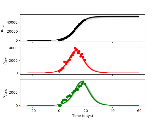
As you can see, most of the generated curves are clustered very tightly, indicating that the estimated variance in the fitting routine is very small for the fitted parameters. It should be mentioned that despite the small uncertainty estimate in the fitting parameters this does not indicate that:

The fitted parameters accurately reflect the real situation (due to differences in model-reality dynamics)
The fitted parameters determined from the non-linear least squares routine found a global minimum instead of a local minimum

Point 1 can be addressed by making a more complex model such as incorporating a model of how people travel around the world (at the expense of time). Point 2 is difficult to address since non-linear least squares fitting does not guarantee a global minimum but a reasonable approach would be to try various starting guess parameters within reasonable limits to see if it converges on a different solution (outside of the variance shown above).

Simple model of real-world data in Python

Short background

Infection model

Solving the differential equation

Data fitting

Error Analysis

Published by Code Wanderer

Leave a comment

Cancel reply

Short background

Infection model

Solving the differential equation

Data fitting

Error Analysis

Share this:

Related

Published by Code Wanderer

Leave a comment

Cancel reply